JET2 Viewer
How to use JET2 Viewer
Input
The user should provide a PDB code. Alternatively, he/she can browse the full list of PDB structures considered in JET2 Viewer and select his/her favorite from the list.
Output
JET2 Viewer provides binding site predictions and residue properties for the query PDB structure. They were computed using the method JET2 (Laine and Carbone, PLoS Comput. Biol., 2015).
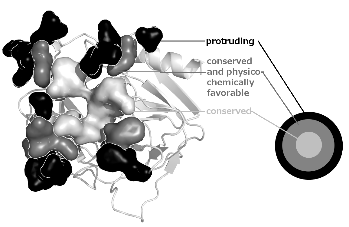
Structure of a binding site predicted by JET2. The site is comprised of three layers : the seed (in light gray), the extension (in gray) and the outer layer (in black):
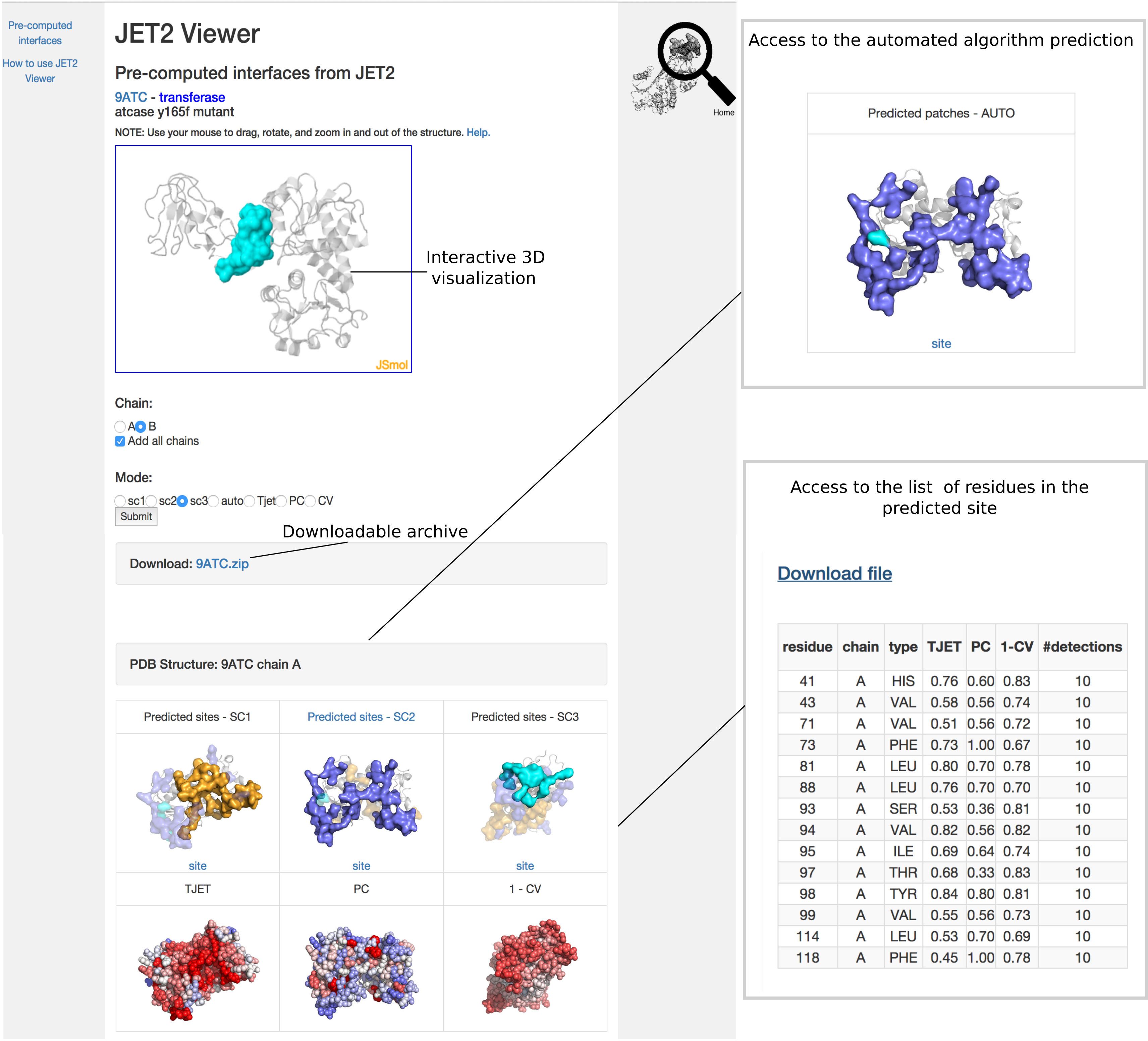
JET2Viewer output page enables to interactively visualize the predicted binding sites and the residue properties on the 3D structure of the query protein. It also provides an intelligent display of the binding sites and the properties mapped onto the 3D structure, and a downloadable archive.
Protein properties computed by JET2
JET2 exploits the sequence and the structure of the query protein to predict binding sites. It uses three biologically meaningful residue descriptors:
- TJET: evolutionary conservation (or trace) computed from phylogenetic trees constructed based on multiple sequence alignments of sequences homologous to the query sequence. JET2 implements an automated sequence selection strategy aiming at spanning the tree of life as much as possible and to guarantee sequence diversity (see Engelen et al., PLoS Comput. Biol., 2009).
- PC: amino acid propensities to be present at an interface taken from (Negi et al., J. Mol. Model, 2007). They were already used in (Engelen et al., PLoS Comput. Biol., 2009).
- CV: circular variance, measuring the local geometry of the surface. CV provides an alternative to solvent accessibility measures, and is described in (Laine and Carbone, PLoS Comput. Biol., 2015).
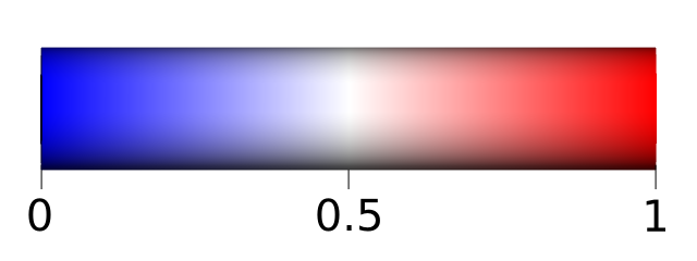
The three scales go from 0 to 1 and follow this scale colors:
Scoring strategies to detect binding sites
JET2 implements three different scoring strategies to predict binding sites:
SC1 (orange) uses all three descriptors. Very conserved residues (TJET only) are detected and grouped to form cluster seeds, which are then extended by using TJET and PC. Residues with high interface propensities (PC) and highly protruding (CV) are finally added to form the outer layer. SC1 is intended to detect diverse protein binding sites and thus corresponds to the general case.
SC2 (purple) uses a combination of TJET and CV for seed detection and extension. This ensures that strong evolutionary signals are captured (TJET) while avoiding residues too buried inside the protein (CV). The outer layer is defined based on PC and CV, as in SC1. SC2 was designed to specifically detect protein interfaces that are located close to or overlap with small-ligand binding pockets.
SC3 (cyan) disregards evolutionary information and rather employs PC and CV for detecting all three layers. The development of SC3 was motivated by the observation that some protein interfaces contain very low conservation signal to none. We expect SC3 to yield consistent predictions for those difficult cases.
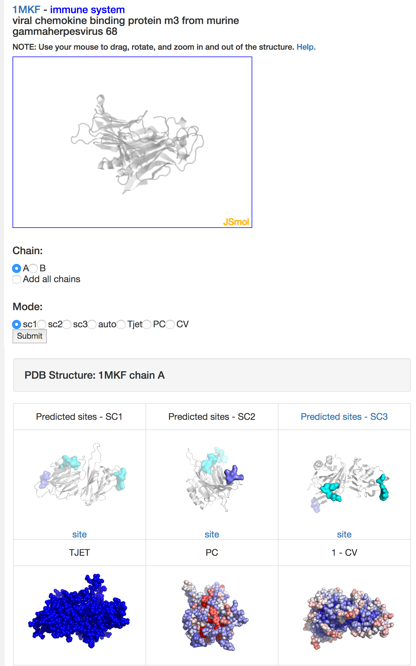
The binding sites predicted by SC1, SC2 and SC3 are displayed as opaque surfaces mapped onto the 3D structure of the query protein (cartoon representation).
List of residues within each binding site
By clicking on the blue link "site", the user can access a table with the list of the residues predicted as interacting and their computed properties : conservation level, interface propensity, structural exposure and the number of times it was detected (among 10 iterations of JET2). Intuitively, a high number of detections expresses that the residue belongs to the core of the interaction.
Binding site predicted by the fully automated clustering algorithm
JET2 also implements a fully automated clustering algorithm. The scoring strategy chosen by this algorithm is highlighted in blue (see Figure above, where SC2 was chosen). The scoring schema automatically selected by JET2 is highlighted in blue (see "SC2 predicted patches" in the figure above). By clicking the blue link, the user can access the complete automatic prediction obtained by combining two complementary scoring schema. In the example above, the patch predicted by SC2 (in purple) was extended with residues coming from SC3 (in cyan).
JSmol window (pull down)
The user can select the chain name and either the site (SC1, SC2, SC3) or the residue property (TJET, PC, 1-CV) that he/she wishes to visualize, and presses "Submit". The selected site can be displayed alone or with all other chains of the complex (added in cartoon), if any. To display all chains, the user checks "Add all chains" and presses "Submit". This allows verifying if the predicted site lies at the interface of two chains in the complex or if it is engaged in the interaction with other potential partners. Residue properties can be displayed for all chains by checking “Add all chains” and by pressing "Submit".
Downloadable archive (pull down)
The archive contains three types of files : PDB, PNG and PML. The PDB files record the 3D coordinates of the query chain and, in the B-factors column, the values computed by iJET2 (10 independent runs of JET2) for each residue: evolutionary conservation (traceMax), physico-chemical properties (pc), circular variance (cv) and prediction score computed as the number of times the residue was predicted as interacting over 10 (clustersOccur), for each scoring strategy (SC1: sc1, SC2: sc2, SC3: sc3, automatic selection: auto). The PNG files display JET2 results (see above). The user can reproduce them and interactively visualize the results by running PyMOL with the PML files as input.
Intelligent display (pull down)
In the three images displaying binding site predictions (on top), the position and orientation of the protein structures in 3D space were pre-computed for each prediction so as to optimize visualization. In the three images displaying the levels of TJET, PC, 1-CV (at the bottom), the structure is in the same position and orientation as that used in SC1, SC2, SC3 respectively. This is because TJET, PC and 1-CV are the major contributors for SC1, SC2 and SC3.
Troubleshooting (no prediction) (pull down)
It can happen that a scoring scheme does not yield any prediction. For example, proteins from viruses may have too few known homologous sequences, so that the evolutionary trace cannot be computed and SC1 cannot predict any binding site. In that case (see image below), the interactive 3D display for SC1 only shows the protein as a grey cartoon, the 2D image for SC1 only displays the other predictions (from SC2 and SC3) as transparent surfaces, and the 2D image representing TJET is completely blue (all trace values at zero).
Troubleshooting (PDB not in the database) (pull down)
Since chains might be very similar in different PDB structures, the analysis of some chains is available through the analysis of homologous ones. In such cases, the user will access a page as follows:
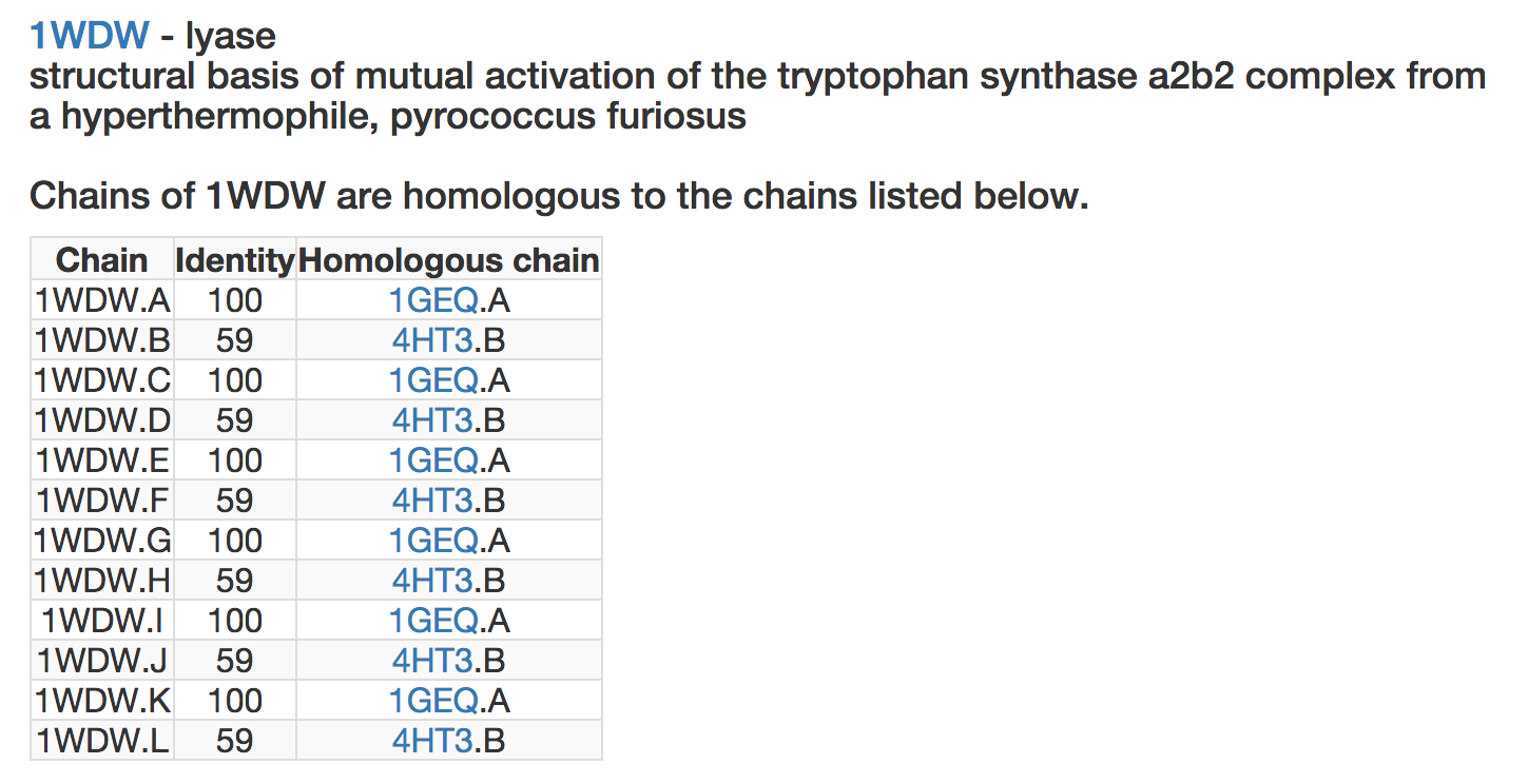
where, for each chain of the query structure (first column), the sequence identity with the proposed homologous chain is indicated (second column) and the analysis of this homologous chain is made available (third column). Note that one might find several alternative analyses for the same chain.
Additional information
- Download JET2 from LCQB website.
- Chains with fewer than 20 amino-acids are not computed by JET2 and not displayed.
- DNA or RNA are not displayed.
- If JET2 is not computed on a chain, we propose an homologous alternative.
- PDB entries were selected using filtering with PISCES according to the following criteria:
- Maximum percentage identity: 40
- Minimum resolution: 0
- Maximum resolution: 3.5
- Maximum R-value: 0.3
- Minimum chain length: 40
- Maximum chain length: 10000
- Skip non-X-ray entries? No
- Skip CA-only entries? Yes
- How do you want to cull PDB? By chains
- Images were generated using PYMOL.
Disclaimer
This server is intended for research purposes only. It is a non-profit service to the scientific community.